10 Skills and Functions to Greatly Improve your Google Sheets Game
Friday September 7, 2018
Many of us work with spreadsheets every day. It’s what allows us to deal with multiple projects at once, each with reams of data. A spreadsheet helps us tame this data — and the better the spreadsheet is laid out and designed, the more it can help us be efficient when processing this data.
Since being promoted to Manager of our support team, I find my nose buried in a spreadsheet far more often than in a system log file. In addition, I’ve found that I can be much more productive by creating well-designed spreadsheets than I could be by turning a screwdriver or tuning some PHP parameters.
There is a basic level of skill that most of us have regarding spreadsheets, but this is just barely tapping the potential of what they can do. Surprisingly, it only takes mastering a few skills and functions to greatly up your spreadsheet game — taking you to the next level in productivity, and wowing your coworkers (which is, admittedly, the real goal here).
My examples use Google Sheets, mostly because it’s what I use daily, but also because everyone using it is using the same version. Almost all of the concepts I discuss can be done in Microsoft Excel, as well, but not only does the method sometimes differ from Google Sheets, it also differs between versions of Excel.
Top 10 Google Sheets Skills and Functions
- Drop-Down Lists with Data Validation
- Conditional Formatting
- Freeze
- Referencing Cells
- VLookup()
- Autofill
- Clean Presentation
- Unique()
- CountIf()
- IfError()
Skill: Drop-Down Lists with Data Validation
Ever wonder how to add a drop-down list to a cell? This is done through Data Validation. Typically, on any spreadsheet I make, I create a “Data” sheet (tab) to hold the various tables that are needed to enable this and other functions, without cluttering up the main workbook.
To add a drop-down list to a cell in Google Sheets (as seen in fig. 1).
- Create a column in the Data tab with a list of all the options you want for the list (see fig. 2).
- Back on the Main tab, right-click on the cell getting the drop-down list.
- Select Data Validation from the bottom of the right-click menu.
- A new window with several options will show up. Don’t be alarmed.
- Click on the Criteria text box, ensuring your cursor is blinking in the box (see fig. 3).
- Now, change tabs to the Data tab and highlight the block of list items.
- Move the Data Validation window if it’s in your way, but don’t close it.
- The Data Validation window will change to a “What data?” window.
- This will display the range of the block you have chosen (see fig. 4).
- i.e. Data!B3:B5
- This means Data tab, from B3 through B5.
- Click OK on the “What data?” window.
- The range you selected will now be in the Criteria field on the Data Validation window that has returned.
- Click Save.
…And that’s it! It really is that simple. Once you’ve done this a couple times, it will become second nature, and then your problem will be restraining yourself from adding too many drop-down lists.
Skill: Conditional Formatting
Conditional Formatting allows you to let the spreadsheet do some of the thinking for you. It formats data in a way that makes it easier to visibly digest by helping you see trends and highlighting specific data points to be better noticed.
For example, I typically use conditional formatting to highlight duplicate items in long, unsorted lists of parts. Many of the part names are similar, so offloading the task of identifying them to the spreadsheet not only helps, but it reduces the chance of human error as well.
There are a number of conditions you can use to configure Conditional Formatting. On the shift schedule I maintain, I use conditional formatting to automatically change a cell color to an employee’s assigned color when it detects their name in the cell. All my shifts show up as cornflower blue, Kirk’s shifts are orange and Zach’s are green.
You can format based on dates — if a person’s membership is expired, mark it red. If it’s due soon, mark it orange, etc. It’s really only limited by your imagination.
In Google Sheets, Conditional Formatting is accessed from the main menu, under Format. Select the range you want to rule to apply to, then select the rule (or use a custom formula), and finally set the format to apply if the rule’s conditions are met.
Figure 5 shows some sample sales data with three Conditional Formatting rules set up for column G. The first rule identifies cells in column G with a value over 100,000 by changing the cell color to green. Next, we identify those cells with a value of over 10,000 with the color orange. Finally, anything equal to 10,000 or less is red.
If you’re paying attention, you might be thinking, why are values over 100,000 green, not orange — since these cells meet the conditions for two different rules. It works because the rules are processed in order. Rules higher on the list trump rules further down. When you mouse over a rule, four horizontal dots show up on the left side and a trashcan on the right. Grab the rule by the four dots to drag it up or down, changing its position. I’m going to let you figure out what the trashcan does — I know you can do it!
In Figure 6, you can see what happens when the rules are out of order. I moved the green rule down (you can see the four dots on the left of the rule that are used to drag the rule up and down), below the orange rule. As you can see, all the previously green cells are now orange, and the green rule has been made useless simply by changing the order.
Skill: Freeze
When working with large sets of data, it’s easy to get lost, especially when the data in several columns is similar. One way to fight this is to freeze the header row. By doing so, the top couple of rows that contain the header are always at the top of your view, and as you scroll down, the rows scroll by, but the header is frozen at the top.
Figure 7 shows the previous example with a frozen header row. Notice how the row numbers skip from two to twenty. No matter how far down you scroll, the header will always be visible.
You can also freeze columns to the left of the sheet, and if you’re feeling adventurous you can freeze both rows and columns.
Skill: Referencing Cells
Most spreadsheet users are somewhat familiar with how to reference cells, called A1 Notation. In this system, a cell is referenced by its column letter, followed by its row number — “B7”, for example. A range of cells is referenced by listing the upper-left cell of the range, followed by the lower-right cell, separated by a colon — “B7:D15”, for example. This example range would be three columns wide and nine rows tall. When we want to duplicate the contents of one cell in another cell, for example, we want the contents of B7 to show up in C12, the formula for C12 would be simply “=B7” where the equal sign indicates a formula to follow, and the formula is simply the cell reference.
Where things get a bit more complex is when we start dealing with relative and absolute cell references. Relative references are what allow the spreadsheet to change cell references when a formula is copied to another cell. For example, E3 is the sum of B3 through D3. The formula for E3 would be:
=Sum(B3:D3)
Because we are using relative cell references, this allows you to copy the formula from E3 down to E4, E5, E6, and so on, with the formulas automatically changing in each new row to add up the elements of that row, and not the original row, row 2. Relative referencing increments the row portion of the cell reference by one when the formula is pasted one row down. It increments by 5 when pasted five rows down, and by -1 when pasted one row above the original. Without this automatic adjustment, when the formula in E3 is copied to E4, rather than add up the elements in the fourth row, it shows the same total as E3 because the formula tells it to display the sum of B3 through D3, rather than B4 through D4. This is true for moving from column to column, as well as row to row.
This feature saves immeasurable time entering formulas into spreadsheets because you can simply set up the formula for one row or column, and copy it to work without modification on your others rows or columns.
In most cases, relative referencing is what you want — but there are situations where you don’t want the reference to change when copying the formula from cell to cell. To demonstrate this, imagine we’re adding tax to subtotals to get the final totals. For this example, we’ll use a mix of relative and absolute cell references. We’ll use an absolute reference to pull the tax rate from its cell, D2, and use it to calculate the tax by multiplying the tax rate by a relative reference to the subtotal. The relative reference to the subtotal will allow us to copy the formula from row to row, using the appropriate subtotal each time, while the tax rate stays fixed. To do this, we add dollar signs to the cell reference to tell the spreadsheet not to change the value, even if a formula is pasted elsewhere. In this case, our tax line for C5 looks like:
=B5*$D$2
Notice how B5 has no dollar signs, while the D2 reference does? The first dollar sign locks down the column part of the reference, while the second locks down the row. The column lock isn’t necessary in this case, but it doesn’t hurt, either. With the column locked, as well, it allows us to use the same formula to generate tax on the cell to the left of it anywhere on the sheet, without losing the tax rate.
If we didn’t use an absolute reference for the tax rate, the first formula we put in would still work, but if we copied it to another row, it would try to pull the tax rate from another row as well. Say we copied the formula from D5 to D6. The tax rate would be blank because it would be referencing D3 since it would be a relative reference. Row 7 would be even worse — the tax rate would be “Total” — and I thought my tax rate was bad…
Anytime you want to lock down the row on a cell or range reference, put a dollar sign in front of the row designator. Do the same with the column designator to lock down the column reference. You’ll find that many of your errors with spreadsheets are caused by incorrectly referencing a cell.
In addition to these different ways to reference a cell, you can also reference cells on different tabs (sheets). I use a Data sheet to hide a lot of my reference tables away from sight. To reference B7 on my Data sheet from another sheet, I use “Data!B7” to reference the cell. The Data! tells the spreadsheet the sheet where the cell can be found.
Function: VLookup()
The Vertical Lookup function, VLookup() is a powerful feature that will help propel your spreadsheets to the next level. This function allows you to populate a cell based on information pulled from another table (often hidden on another tab, or even on another spreadsheet, but the latter would require the ImportRange() function, which you can investigate if you’re feeling adventurous).
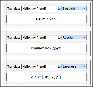
The language drop-down list is generated using Data Validation with the first column of the language list on the Data tab.
The translation cell is generated by embedding a VLookup() function within the GoogleTranslate() function
The GoogleTranslate() function has three elements: the source text, the source language abbreviation, and the target language abbreviation, resulting in the following formula structure:
=GoogleTranslate(
The final translation formula looks like:
=GoogleTranslate(D3,”en”,VLookup(F3,Data!B3:C66,2,True))
In this example, D3 is the source text, “Hello my friend!” The source language abbreviation is “en” for English, and VLookup() is used to convert the Language name chosen in the dropdown, F3, to its abbreviation.
The VLookup() function has four elements: the search key, the range, the index, and the optional is_sorted boolean (boolean is just a fancy word meaning it is either TRUE or FALSE). Using the VLookup() function looks like:
=VLookup(
In our example, the function is embedded within the GoogleTranslate() function, with the VLookup() portion looking like:
VLookup(F3,Data!B3:C66,2,True)
Here, the full name of the language chosen in the dropdown list, cell F3, is used as the search key. In the first translator, I have “Swedish” selected as this key.
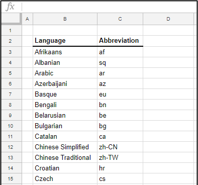
The next field is the range, Data!B3:C66. As we learned in the Variables section, Data! references the Data tab, and B3:C66 refers to columns B and C on the Data tab, from row 3 through row 66. Figure 9 shows this table of the possible languages listed by full name in column B and the associated abbreviation in column C. Make sure not to include the table headers in the range.
The index is the column number of the result we want to return. Note that this index is in relation to the range chosen in the second element. In our example, I use “2” to reference the second column in the range, column C. What is happening in simple terms is the spreadsheet looks at our table on the Data tab and looks down the first column for an entry that matches our key, “Swedish.” Once this key is found, it looks across to the index column, the second column in the range — column C — and finds the abbreviation associated with “Swedish” — “sv” (for Svenska, Swedish for “Swedish”). The VLookup() function then returns “sv” to the GoogleTranslate() function, which allows the translation to happen.
To show a more complicated example, I recently used VLookup() to help fill out a spreadsheet dealing with access to various security doors in our facility. We have four doors secured with a badge reader and five levels of access, with no access represented by a blank entry. Figure 10 shows my lookup table on the Data tab and figure 11 shows the result of several VLookup() functions at work on a lookup table that is more than just two columns.In figure 11, each of the four doors has a slight variation of the VLookup() function. They end up looking like:
Front 1 =VLookup(F4,Tables!G$4:K$8,2,TRUE)
Front 2 =VLookup(F4,Tables!G$4:K$8,3,TRUE)
DC =VLookup(F4,Tables!G$4:K$8,4,TRUE)
Dock =VLookup(F4,Tables!G$4:K$8,5,TRUE)
One key detail to note is the addition of dollar signs “$” to the row element of the range in the VLookup() functions. This is important because if I just copied the functions from one row to the next without them, the range would automatically increment, causing errors after a few rows. This also happens when Autofill is used to replicate the rows quickly (Autofill will be discussed next), but again this can be avoided by using dollar signs to lock down the range of the VLookup().
You’ll notice the only difference between the entries for each door is the third element, the index. This tells the spreadsheet from which column within the lookup range to retrieve the value.
Skill: Autofill
Google Sheets has an autofill feature that can be used to quickly duplicate cells, or continue sequences and patterns, saving you a lot of time that would be wasted on tedious data entry. If you haven’t been using this feature, you certainly will be once you learn how it works.
The simplest Autofill feature is duplication. Say you have a list of questions in one column and answers in the next — but you don’t have any answers yet. Rather than leaving the Answers fields blank, you want to pre-populate the field with a placeholder, “
You can use this to fill down, or right. You can do both, but you have to do one at a time — Fill down, let go and grab the dot again, this time with the whole row still highlighted and fill right. The reverse order works as well (right, then down).
In addition, you can start with more than one cell. Say you have a column next to the Answers column that shows Answered by whom. Enter “
Granted, the times you’ll need to use this to duplicate text is likely somewhat limited — but it becomes much more useful when you realize you can duplicating formulas, not just text or numbers. When duplicating formulas, keep in mind what we learned about absolute and relative cell references — especially the use of the dollar sign. This will lock the references so they don’t increment from row to row. Some situations will call for this, and others won’t. I find I often end up with a mix of relative and absolute references in my functions (like the door access example in the VLookup() section).
The real power of Autofill is shown by its ability to iterate sequences. Say you want to number your questions 1 through 15. Simply fill in the first two numbers, highlight both cells and pull the blue dot down until you’ve highlighted 15 cells. When you let go, you’ll see the sequence continued into the area highlighted, leaving you with the number 1 through 15.Now let’s try something a bit tricker — you want to count by twos. If you want odd numbers, leave the 1 in the first cell and replace the 2 with a 3. Highlight the first two cells again and drag down — you’ll see the numbers 1 through 15 have now been replaced with the odd number 1 through 29.
You don’t have to start with 1, either. Start at 23 and count upwards (or downwards), if it’s what you need. Do you double-space? Start with 1 (or another number) and select that cell and the empty cell below it. Drag down, and you’re numbering every other row (see figure 12).
Google Sheets will also detect patterns in your cell for Autofill. Start with “word1” and “word2” and you can use Autofill to further the sequence with “word3,” “word4,” etc. In my role as a support manager, I use this to populate lists of IP addresses (see figure 13) frequently.
If the spreadsheet doesn’t detect a number in the highlighted fields, in most cases it will simply repeat the sequence of highlighted fields over and over again. With a single field, this simplifies to basic duplication, but if you enter “duck,” “duck,” “duck,” and “goose” into four cells and Autofill them (see figure 14), you will see that pattern repeated.
In that last example, I said “in most cases” because there are a few exceptions. Google Sheets used to be able to reference a Google Labs feature called Google Sets. Google sets allow you to start listing items from a set and Autofill cells with additional members of the set. You could then use a function called GoogleLookup() to pull information about the items in the set. An example I saw used elements as the set (starting with Hydrogen, Helium, and Lithium). Additional columns were filled in by referencing (similar to a VLookup() function, but referencing data from Google Sets). These additional columns displayed each element’s Atomic Weight, Atomic Number, and Melting Point. To be honest, I’m not sure if I’d get much use of that feature — but it was great for showing off! Unfortunately, this feature was removed several years ago.
Why bring up an outdated feature? Well, imagining how Autofill used to work with sets will help understand how Autofill works with dates and times. Type the name of a month of the year, highlight it and drag down. You will see that instead of repeating that word, it filled in the rest of the months, in order. If you go past 12 cells, it will start repeating. You can do the same with the days of the week (see figure 15).
Dates can be Autofilled using a variety of formats (any format recognized by the spreadsheet as a date). By default, if you start on a specific date and use the one cell to Autofill, it will increment each cell by one day. If you want to increment monthly, or weekly, enter the first two elements of the sequence and select those two cells to Autofill from (see figure 16).
Times Autofill in a similar way. By default, the spreadsheet will use the 24-hour format, but adding “AM” or “PM” will force it to the 12-hour format for our delicate American sensibilities. Start with “12:00 PM” in a cell, and it will Autofill times in one-hour increments, using the 12-hour format. Want to count in 15-minute increments, fill in the second cell with “12:15 PM” and start your Autofill with the first two cells to achieve this (see figure 17).
Skill: Clean Presentation
This last skill is much more general than the previous skills discussed here. It is more of a collection of ideas, any number of which you can choose to incorporate in your own spreadsheets in order to clean up the presentation.
By default, spreadsheets can daunting blocks of raw data — and it doesn’t help that many of us have picked up some bad habits along the way. It’s amazing to see the difference a few small changes make to the look and feel of a spreadsheet.
- Provide a buffer.
- The first thing I tend to do with a new, blank spreadsheet is resize the first column to the same width as the height of each row (21 pixels). I then start my spreadsheet from B2, which provides a nice buffer around my tables, keeping them from running into the edges, while not giving up too much valuable work area.
- Size your columns so your data has breathing room, without losing valuable space.
- Align your data.
- Right-justify numbers, left-justify everything else.
- Fight the urge to always center your data.
- This is not an absolute rule. Sometimes the presentation looks better with different justification — use your best judgment.
- One big exception to the no-center suggestion is table titles. Merge the top row of cells above the header row into one and center the title in a large font.
- Choose your colors wisely.
- Try to limit yourself to two or three colors on a page.
- Use muted colors, unless you’re trying to highlight something to make it more noticeable.
- In the example below, I’ve changed the Conditional Formatting of the sales numbers to change the text color, not the cell color. I prefer more subtle indicators, but sometimes bold is what’s needed. Format accordingly.
- Choose complementary colors — see the colors used in Format ➡ Alternating Colors for examples of muted colors that go well together.
- Format ➡ Alternating Colors can be used to highlight the header row and put a light color on alternating rows below the header to help follow a line across the page.
- I tend to use light greys and light blues as my go-to colors. If I need to venture beyond those colors, I choose a color and match it with a color just above or below it in the color-picker. Go up and down, not left and right — unless you’re working with greys.
- Avoid overuse of borders.
- I will often limit borders to a single line separating the header column from the data — however, this is unnecessary when you use a bolder cell color to highlight the header or freeze the header column.
- I also tend to frame the table when I have more than one small table on the same tab, often with a two or three pixel wide border.
Compare the before and after spreadsheets. It’s amazing what a few small changes can do.
Which one would you work with? Which one would you like to present to a large audience?
Function: Unique()
The Unique() function takes a range of data and returns a list with all duplicates removed. Elements are returned in the order they are encountered, so I often embed this function within a Sort() function to return a sorted list.
I frequently use this function for inventory tracking. Say there is a list of components for 40 servers, one per row, with the F column listing the server’s CPU. If we want a list of the different types of CPUs in use by these 40 servers, our function would look something like:
=Unique(F3:F42)
In this example, F3:F43 is the range covering the list of CPUs for the 40 servers. In this case, let’s say there were only four different types of CPU in use. The first type encountered would be displayed in the cell with the above formula. The following unique CPUs would fill out the three cells below.
If you want a sorted list, the Unique() function could be placed in a Sort() function:
=Sort(Unique(F3:F42), 1, TRUE)
To cover how Sort() works, in simple cases like this, the first element is the range to sort. The second element is the column within that range to sort — in our case, there is only one column, so we use “1.” Finally, a boolean value to represent if we want the list sorted in ascending order, or not. Sort() has a few more options to play with if you want, but those are the basics.
Function: CountIf()
The function CountIf() counts the number of cells that meet a definable condition within a range of cells. I find I often use it in conjunction with Unique() to make a table summarizing how many of each part are in use. Using the example from the Unique() description, once a list of unique CPUs is generated, I use CountIf() to count how many servers have each CPU type.
Say N5 is where we start our unique CPU list, generated from the range F3:F43. Since there are 4 different CPUs, these are listed in N5 though N8. I use the next column, M, to show counts of each of these CPUs. The formula for M5 would be:
=CountIf(F$3:F$34, N5)
Where the first element is the range in which to count (notice the absolute row references), and the second element is the condition that triggers a count if it is met. In our example, the range is again F3:F43 — the CPU list for the 40 servers, and the condition is N5, the first CPU on the unique list.
You can use more advanced criteria than simply matching, too. If I want to count how many values in a list are greater than 20, I’d use “>20” (including the quotation marks) as the criteria for CountIf().
Function: IfError()
IfError() is a simple function that helps clean up expected errors in a spreadsheet. Expected errors often turn up when some data has yet to be entered, and functions referencing that empty cell throw an error because it need some data to process, or it can be something as simple as dividing by zero.
Some common errors you’ll see will be #DIV/0!, #VALUE, #REF!, and #NUM!. Wrapping your function in IfError() can suppress these errors. The function:
=IfError(B2/B3, “Oops!”)
will return whatever the formula in the first element, here B2/B3, would normally return unless the return value is an error. In most cases, it would return the result of B2 divided by B3. However, if B3 happens to be a zero, the formula would return the error, #DIV/0! The IfError detects the error, suppresses it, and returns the 2nd (optional) element — in this case, “Oops!” If you leave out the second element, the error is still suppressed, if one is returned by the formula in the first element, but nothing is returned — the cell is left blank.
While this is a useful tool to keep errors from mucking up your nice, neat spreadsheet, it can make troubleshooting mistakes difficult. Keep that in mind when putting a spreadsheet together, and maybe add the IfError() wrappers after you’re confident in your work.